Low-precision formats such as MXFP8 and NVFP4 promise substantial throughput gains for LLM pretraining. But a quantized run also ends at a higher loss, and how much higher depends on the model size, the token budget, and which operations are quantized. A predictive scaling law is therefore essential for choosing a quantization recipe and its configuration before committing compute to a large run.
This post follows how we built such a law. We first decompose existing 4-bit recipes to find where their gains come from, which motivates mixed precision. We then develop scaling laws for mixed precision at two levels, across the forward and backward passes and across layers, and use them to find the compute-optimal precision allocation.
Summary
- Recipe decomposition. Forward-pass quantization causes most of the loss increase in existing 4-bit recipes, and even the best one still trails BF16.
- Forward–backward mixed precision. Modeling a persistent optimization error for each pass achieves lower held-out MSE than the Quartet law when extrapolating to both larger models and more data.
- Layer-wise mixed precision. A simple extension predicts mixed configurations accurately, and shows that which blocks stay in higher precision matters far more in the backward pass.
- Compute-optimal allocation. The optimal precision increases with the compute budget, and the backward pass keeps low precision longer than the forward pass.
Where Do the Gains of 4-Bit Recipes Come From?
Existing FP4 recipes combine several techniques and are usually evaluated as complete configurations. We decompose two of them, the NVIDIA NVFP4 recipe and Quartet II, into forward and backward components. In the forward pass, the NVFP4 recipe shares scales across 16×16 weight blocks (2D scaling), while Quartet II uses 1×16 blocks with 4/6 scaling, which picks the lower-error of two candidate scales per block. In the backward pass, the NVFP4 recipe uses stochastic rounding (SR) and randomized Hadamard transforms (RHT), while Quartet II uses MS-EDEN for unbiased matrix multiplication.
| Forward | Backward | Val. loss | Increase over BF16 |
|---|---|---|---|
| BF16 | BF16 | 3.245 | – |
| BF16 | MS-EDEN | 3.257 | +0.36% |
| BF16 | RHT + SR | 3.255 | +0.32% |
| BF16 | SR | 3.268 | +0.72% |
| 4/6 + 1D scaling | BF16 | 3.275 | +0.94% |
| 4/6 + 1D scaling | MS-EDEN (Quartet II) | 3.280 | +1.07% |
| 4/6 + 1D scaling | RHT + SR | 3.282 | +1.14% |
| 2D scaling | BF16 | 3.284 | +1.22% |
| 2D scaling | RHT + SR (NVFP4 recipe) | 3.291 | +1.41% |
Table 1. Validation loss of a 430M-parameter Qwen3 model trained on 12.8B tokens, with each pass quantized to NVFP4 using the listed technique.
We found that forward-pass quantization dominates the loss degradation. Quantizing only the backward pass raises the loss by 0.32–0.72%, while quantizing only the forward pass raises it by 0.94–1.22%, and most of Quartet II’s advantage over the NVFP4 recipe comes from its forward pass. Even the strongest recipe still leaves a noticeable gap to BF16.
Closing this gap without giving up most of the speedup calls for mixed precision pretraining, which keeps the most sensitive computation in higher precision. Mixed precision arises at two levels: across the forward and backward passes, and across layers. The next two sections develop a scaling law for each.
Mixed Precision Across the Forward and Backward Passes
Persistent Optimization Error
Existing laws model quantization only through effective counts: forward quantization shrinks the effective parameter count, and in the Quartet law, backward quantization shrinks the effective token count. Both can be offset by scaling up, but quantized training also leaves optimization error that does not go away with more training: weights can oscillate across rounding boundaries in the forward pass, and gradient estimates can be biased in the backward pass.
With weights \(\theta_t\) and quantized weights \(\hat\theta_t = Q(\theta_t;\psi_f)\) over \(T\) training steps, the loss gap splits as
\[\mathbb{E}_{J,\theta_J}\big[\mathcal{L}_N(\hat\theta_J)\big] - E = \underbrace{\big(\mathcal{L}^*_{N,\psi_f} - E\big)}_{\text{capacity gap}} + \underbrace{\big(\mathbb{E}_{J,\theta_J}\big[\mathcal{L}_N(\hat\theta_J)\big] - \mathcal{L}^*_{N,\psi_f}\big)}_{\text{optimization gap}},\]where \(J\) is uniform over the \(T\) steps, \(\mathcal{L}^*_{N,\psi_f}\) is the best loss the quantized model can reach, and \(E\) is the irreducible loss. Backward quantization changes only the updates, so the capacity gap depends only on \(N\) and \(\psi_f\).
For updates \(\theta_{t+1} = \theta_t - \eta\,\hat g_t\) with gradient estimates \(\hat g_t\) computed at \(\hat\theta_t\) under \(\psi_b\) and bias \(b_t\), standard assumptions (convex loss, bounded moments, \(\eta = c/\sqrt{T}\)) give
\[\begin{aligned} \mathbb{E}_{J,\theta_J}\big[\mathcal{L}_N(\hat\theta_J)\big] - \mathcal{L}^*_{N,\psi_f} &\le \underbrace{\frac{1}{2\sqrt{T}}\left[\frac{R_1}{c} + \frac{c}{T}\sum_{t=1}^{T}\mathbb{E}\Vert \hat g_t\Vert ^2\right]}_{\text{(a)}\;O(T^{-1/2})} \\ &\quad+ \underbrace{G\left(\frac{1}{T}\sum_{t=1}^{T}\mathbb{E}\Vert \hat\theta_t - \theta_t\Vert ^2\right)^{1/2}}_{\text{(b)}\;O(1)} + \underbrace{\frac{1}{T}\sum_{t=1}^{T}\mathbb{E}\big[\Vert b_t\Vert \,\Vert \theta_t - q^*\Vert \big]}_{\text{(c)}\;O(1)}, \end{aligned}\]where \(q^*\) is the best quantized solution, \(R_1 = \mathbb{E}\Vert \theta_1 - q^*\Vert ^2\), and \(G\) bounds the gradient norm. Each term motivates a term in our law:
- (a) shrinks with more steps, i.e., more tokens, giving the effective token count \(\rho_D(\psi_b)D\).
- (b) comes from forward quantization error, which need not vanish (quantized iterates can cycle forever), giving \(\epsilon_f(\psi_f)\).
- (c) comes from backward gradient bias, which can persist, giving \(\epsilon_b(\psi_b)\).
where \(\rho_N\) and \(\rho_D\) rescale \(N\) and \(D\). Without the \(\epsilon\) terms, this is the Quartet law.
Does It Extrapolate?
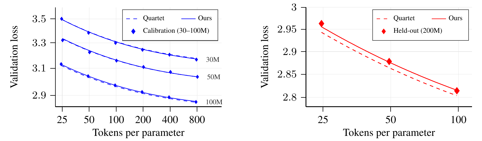
We evaluate on two grids: 84 published Quartet runs of Llama-style models (30M–200M parameters, 25–800 tokens per parameter) and 375 of our own Qwen3 runs (280M–910M parameters, 12.8B–35.8B tokens) covering BF16, MXFP8, and the NVFP4 components from Table 1 in every forward–backward combination. We fit each law on smaller models or token budgets and predict the held-out larger ones.
| Extrapolation | Law | Quartet grid MSE | Quartet grid MAPE | Qwen3 grid MSE | Qwen3 grid MAPE |
|---|---|---|---|---|---|
| Model size | Quartet | 1.6e-4 | 0.386% | 8.4e-6 | 0.076% |
| Model size | Ours | 1.4e-5 | 0.096% | 5.3e-6 | 0.059% |
| Data | Quartet | 9.0e-5 | 0.234% | 2.7e-5 | 0.121% |
| Data | Ours | 5.1e-5 | 0.217% | 6.1e-6 | 0.064% |
Table 2. Held-out loss prediction error on quantized runs.
Our law is more accurate in every setting, reducing MSE by 1.6× to 11×. The plots below show the largest gap: on the Quartet grid, both laws fit the 30M–100M calibration runs almost equally well, but only ours tracks the held-out 200M runs, where the Quartet law underestimates the loss.
Ablations confirm that both error terms help, with the forward term doing most of the work. Removing \(\epsilon_f\) raises the geometric-mean held-out MSE from 1.23e-5 to 3.76e-5, close to the Quartet law’s 4.27e-5, while removing \(\epsilon_b\) raises it to 1.34e-5.
Mixed Precision Across Layers
A Law for Layer-Wise Mixing
Practical recipes often keep some Transformer blocks in higher precision. To predict such configurations, we assign a low-precision configuration \(\psi_2\) to a fraction \(p\) of the blocks and a high-precision one \(\psi_1\) to the rest, and model the loss as
\[L = (L_2 - L_1)\,p^{\gamma_S} + L_1,\]where \(L_1\) and \(L_2\) are the losses of the two uniform configurations predicted by our law from the previous section, and the exponent \(\gamma_S\) captures the block selection strategy \(S\). A good strategy quantizes the least sensitive blocks first, keeping the loss near \(L_1\) for longer, which shows up as a larger \(\gamma_S\).
Prediction Accuracy
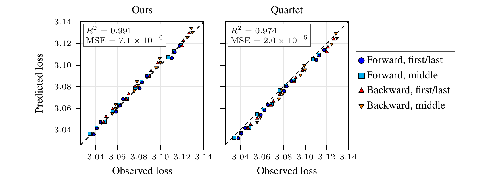
We test MXFP8/NVFP4 mixing on Qwen3 in each pass, with two strategies: keeping the first and last blocks in MXFP8, as in practical NVFP4 recipes, or keeping the middle blocks. Fitting \(\gamma_S\) on the three smaller models and predicting the held-out 910M model, the law matches the observed losses closely (\(R^2=0.991\)). With endpoints from the Quartet law instead, the predictions consistently underestimate the loss and the MSE nearly triples.
Block Placement Matters More in the Backward Pass
The fitted exponents also show where it matters which blocks stay in higher precision.
| Pass | Strategy | \(\gamma_S\) | Gap incurred at \(p=0.5\) |
|---|---|---|---|
| Forward | First/last | 1.10 | 46.7% |
| Forward | Middle | 1.00 | 50.1% |
| Backward | First/last | 1.60 | 33.0% |
| Backward | Middle | 0.50 | 70.7% |
Table 3. Fitted exponents and the fraction of the loss gap between MXFP8 and NVFP4 incurred with half the blocks in NVFP4.
In the forward pass, placement barely matters. Both strategies have \(\gamma_S \approx 1\), so the loss grows roughly linearly with the fraction of NVFP4 blocks, and quantizing half of them incurs about half of the gap either way.
In the backward pass, placement makes a large difference. Keeping the first and last blocks in MXFP8 gives \(\gamma_S = 1.60\), so quantizing half of the blocks incurs only 33.0% of the gap. Keeping the middle blocks instead gives \(\gamma_S = 0.50\) and incurs 70.7% of the gap, more than twice as much. The common practice of keeping the first and last blocks in higher precision therefore pays off mainly in the backward pass, and the choice of blocks deserves the most care there.
Compute-Optimal Precision Allocation
Setup
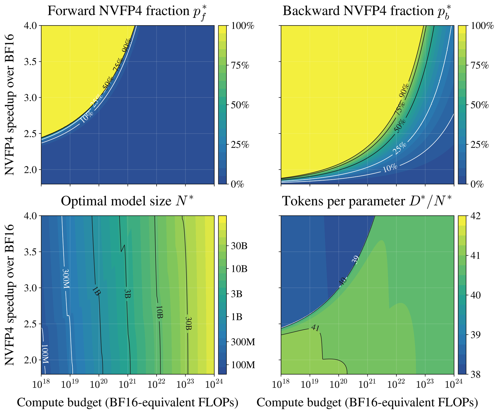
We combine the two laws with a cost model in which the forward and backward passes account for one third and two thirds of training FLOPs, and each format has a hardware speedup over BF16. Under a fixed compute budget, we then solve for the compute-optimal model size, token count, and fraction of NVFP4 blocks in each pass, with first/last block selection. Figure 1 shows the solution.
Optimal Precision Increases with the Budget
Fixing the NVFP4 speedup and increasing the budget, the optimal NVFP4 fractions in both passes decrease. At a 3× NVFP4 speedup, for example, the forward pass switches to MXFP8 around \(10^{20}\) FLOPs and both passes around \(5\times10^{22}\) FLOPs, with layer-wise mixing making the backward switch gradual. Prior precision scaling laws instead predict a budget-independent optimal precision. The difference comes from the persistent error: as the budget grows, the model- and data-dependent loss terms shrink while the persistent error stays, so the lower error of higher precision eventually outweighs the compute it costs.
The Backward Pass Should Go to Low Precision First
The backward pass keeps NVFP4 up to much larger budgets than the forward pass, for three reasons. It accounts for two thirds of training FLOPs, so each NVFP4 block saves more compute. Its larger \(\gamma_S\) under first/last selection, from the previous section, means NVFP4 blocks cost a smaller share of the loss gap. And the fitted persistent error of NVFP4 relative to MXFP8 is about half as large in the backward pass as in the forward pass. With a limited budget for higher precision, it should go to the forward pass first.
Conclusion
Decomposing existing 4-bit recipes shows that the forward pass dominates the loss of quantized pretraining and that a gap to BF16 remains, which calls for mixed precision. At the level of passes, modeling the persistent optimization error from forward and backward quantization makes loss prediction substantially more accurate. At the level of layers, a simple law predicts mixed configurations and shows that block placement matters most in the backward pass. Together, they predict that the compute-optimal precision increases with the compute budget: as training runs grow, low precision is best spent on the backward pass, while the forward pass returns to higher precision first.
The paper is on arXiv.